
 Bluesky
Movie data analysis
Intro
I decided to dig into my film-watching habits as a data exploration exercise.
I used to watch a lot of films. And while watching movies is no longer a significant pastime for me, it was fun at the time. Aside from the apparent interest in the films themselves, the extensive pop-culture knowledge I gained acted as some social currency. Back then, I would make the (outrageous) claim that I’d probably watched every film that would ever come up in casual conversation.
After each film I watched, I would immediately then give it a rating out of 10 on IMDb. I didn’t think I was a critic - this was just the best way to get recommendations for even more films in the pre-Netflix era. A pleasant side effect of this ritual is that I now have a record of every movie I ever watched in that time, along with when I watched it, what I thought of it and other metadata. With the help of IMDb’s data export feature, I now have my hands on my own little cinematic time capsule ! This blog post aims to take a look at that data in pursuit of insights.
Some of the questions I want to answer
- What were my viewing habits?
- Did I have interesting or unusual tastes, or was I poser?
- How do my ratings compare to other IMDB users?
Housekeeping notes
- I’ve written this post as a Jupyter notebook, with inline code snippets, and exported as markdown (you can see the original notebook here).
- If you’re not familiar with Jupyter, it’s a notebook environment that enables literate programming.
- I will keep my dataset private (see here for why !), but you can grab your own dataset here.
- I’ll be using the terms ‘movies’ and ‘films’ interchangably throughout. I’m sure there’s some technical distinction, but generally I think the former is an Americanism.
- I’ll be making use of the two canonical Python libraries:
pandas(for data analysis) andseaborn(for visualisation).
Setup
First, some (non-interesting) initial setup
# Imports
import pandas as pd
import seaborn as sns

# Configuration
pd.options.display.float_format = '{:.1f}'.format
pd.options.mode.chained_assignment = None  # default='warn'
sns.set(rc={'figure.figsize':(16,12)})
# Let's read in the data
INPUT_FILE_ENCODING = "ISO-8859-1"
input_data_path = "imdb_ratings.csv"
imdb_data = pd.read_csv(input_data_path, encoding=INPUT_FILE_ENCODING)
# ... and preview it
imdb_data.head(1)
| Const | Your Rating | Date Rated | Title | URL | Title Type | IMDb Rating | Runtime (mins) | Year | Genres | Num Votes | Release Date | Directors | |
|---|---|---|---|---|---|---|---|---|---|---|---|---|---|
| 0 | tt0100053 | 1 | 2013-01-18 | Loose Cannons | https://www.imdb.com/title/tt0100053/ | movie | 4.9 | 94.0 | 1990 | Action, Comedy, Crime, Thriller | 4394.0 | 1990-02-09 | Bob Clark |
# Let's perform some minor cleanup of the data
# ... filtering out the non-movie entries (TV shows, video games, etc.)
movies = imdb_data[imdb_data['Title Type'] == 'movie']
# ... and formatting the date field
movies['Date Rated'] = pd.to_datetime(movies['Date Rated'])
Great, now we’re ready to explore!
Summary
Next, let’s look at some summary statistics to get an overview of the dataset. Think of this as a tl;dr.
We have different datatypes in our dataset, so we’ll summarize these separately:
# Numeric fields
movies.describe()
| Your Rating | IMDb Rating | Runtime (mins) | Year | Num Votes | |
|---|---|---|---|---|---|
| count | 869.0 | 868.0 | 868.0 | 869.0 | 868.0 |
| mean | 5.1 | 6.8 | 111.6 | 2000.3 | 273587.3 |
| std | 2.2 | 1.1 | 22.2 | 11.7 | 320816.3 |
| min | 1.0 | 2.1 | 60.0 | 1941.0 | 88.0 |
| 25% | 4.0 | 6.2 | 96.0 | 1995.0 | 65191.5 |
| 50% | 6.0 | 6.9 | 107.0 | 2002.0 | 166071.5 |
| 75% | 7.0 | 7.6 | 123.2 | 2009.0 | 361292.5 |
| max | 10.0 | 9.3 | 210.0 | 2018.0 | 2301033.0 |
# Object fields
movies.describe(include=[object])
| Const | Title | URL | Title Type | Genres | Release Date | Directors | |
|---|---|---|---|---|---|---|---|
| count | 869 | 869 | 869 | 869 | 868 | 868 | 869 |
| unique | 869 | 867 | 869 | 1 | 300 | 835 | 533 |
| top | tt0277371 | The Omen | https://www.imdb.com/title/tt0061695/ | movie | Comedy | 2007-06-12 | Steven Spielberg |
| freq | 1 | 2 | 1 | 869 | 56 | 3 | 14 |
OK, so I’ve watched (at least) 869 films. A quick glance of the IMDb website shows that figure includes 96 of their Top 250 films (and also 6 of their bottom 100 films). It goes without saying that 869 is a lower-bound for my total lifetime count, since I’ve continued to watch films but not rate them, and of course I watched films before I discovered IMDb.
Questions
Now, let’s ask some questions of the data
What do my ratings look like?
Zooming in on just the ratings, I’ll use a histogram to visualise the frequency distribution:
sns.catplot(data=movies, kind="count", x='Your Rating')
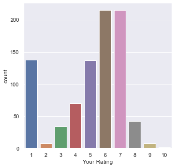
A lot more ‘1’ ratings than I expected! I must have been hard to please.
We can also plot the KDE for an estimate of the probability density (the y-axis here is ‘density’):
sns.set(rc={'figure.figsize':(8,6)})
sns.distplot(a=movies['Your Rating'], bins=range(1,11))
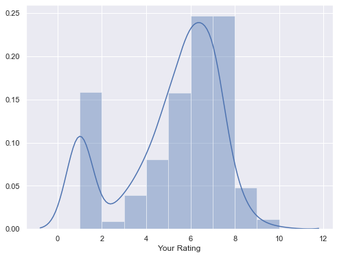
It look’s like about half of my ratings were either a 6 or a 7 out of 10. How very diplomatic(!)
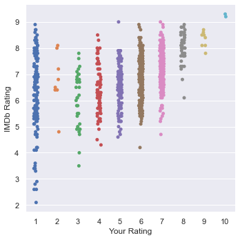
How do my ratings compare to other IMDB users?
Let’s calculate the Spearman’s rank correlation coefficient, as a measure of Inter-rater reliability. It’s values range from -1 to 1 (fully opposed to identical). We’re using Spearman here because our data (Ratings out of 10) is ordinal.
movies['Your Rating'].corr(movies['IMDb Rating'], method='spearman')
0.4413428717210753
Intuitively, a weak positive correlation.
Let’s visualize this relationship. I’ll use a catplot here to get around the problem of representing categorical data with a scatter plot
sns.catplot(x='Your Rating', y='IMDb Rating', data=movies)
What day did I tend to watch films?
# non-interesting date formatting
movies['Weekday'] = movies['Date Rated'].dt.day_name()
movies['WeekdayNumeric'] = movies['Date Rated'].dt.weekday
movies = movies.sort_values('WeekdayNumeric', inplace=False)
# Let's plot
sns.catplot(x="Weekday", kind="count", data=movies, height=5, aspect=12/9)
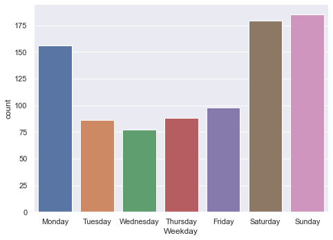
The weekends of course make sense. But Monday is unexpected - TGIM?
What year did I watch the most films?
movies['YearWatched'] = movies['Date Rated'].dt.year
sns.catplot(x="YearWatched", kind="count", data=movies, height=6, aspect=12/9)
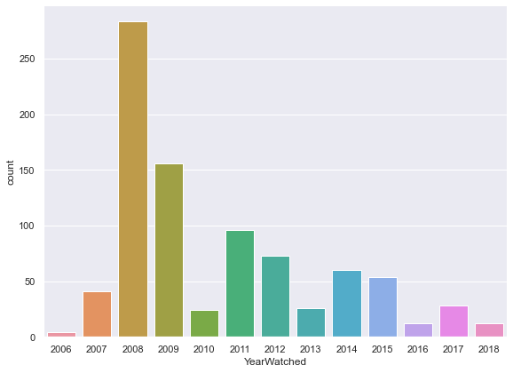
2008, clearly! That was about 1 film per weekday! It looks like the intensity waned over time: 2010, in contrast, was my first year in college - studying obviously took precedence!
What is the least well-known film I’ve watched? (by number of ratings by other users)
movies.sort_values('Num Votes').head(1)
| Const | Your Rating | Date Rated | Title | URL | Title Type | IMDb Rating | Runtime (mins) | Year | Genres | Num Votes | Release Date | Directors | Weekday | WeekdayNumeric | YearWatched | |
|---|---|---|---|---|---|---|---|---|---|---|---|---|---|---|---|---|
| 878 | tt0097073 | 1 | 2007-08-11 | Code Name Vengeance | https://www.imdb.com/title/tt0097073/ | movie | 4.1 | 96.0 | 1987 | Action, Adventure, Drama, Thriller | 88.0 | 1987-12-31 | David Winters | Saturday | 5 | 2007 |
Frankly, this movie looks terrible. Thankfully, I don’t remember watching it (!)
What is the most well-known film I’ve watched? (by number of ratings by other users)
movies.sort_values('Num Votes', ascending=False).head(1)
| Const | Your Rating | Date Rated | Title | URL | Title Type | IMDb Rating | Runtime (mins) | Year | Genres | Num Votes | Release Date | Directors | Weekday | WeekdayNumeric | YearWatched | |
|---|---|---|---|---|---|---|---|---|---|---|---|---|---|---|---|---|
| 100 | tt0111161 | 10 | 2007-08-11 | The Shawshank Redemption | https://www.imdb.com/title/tt0111161/ | movie | 9.3 | 142.0 | 1994 | Drama | 2301033.0 | 1994-09-10 | Frank Darabont | Saturday | 5 | 2007 |
This one needs no introduction!
What was the least liked film I’ve watched? (by ratings by other users)
movies.sort_values('IMDb Rating').head(1)
| Const | Your Rating | Date Rated | Title | URL | Title Type | IMDb Rating | Runtime (mins) | Year | Genres | Num Votes | Release Date | Directors | Weekday | WeekdayNumeric | YearWatched | |
|---|---|---|---|---|---|---|---|---|---|---|---|---|---|---|---|---|
| 704 | tt0473024 | 1 | 2007-08-11 | Crossover | https://www.imdb.com/title/tt0473024/ | movie | 2.1 | 95.0 | 2006 | Action, Sport | 8910.0 | 2006-07-22 | Preston A. Whitmore II | Saturday | 5 | 2007 |
Ah, this doesn’t look that bad
What was the most liked film I’ve watched? (by ratings by other users)
movies.sort_values('IMDb Rating', ascending=False).head(1)
| Const | Your Rating | Date Rated | Title | URL | Title Type | IMDb Rating | Runtime (mins) | Year | Genres | Num Votes | Release Date | Directors | Weekday | WeekdayNumeric | YearWatched | |
|---|---|---|---|---|---|---|---|---|---|---|---|---|---|---|---|---|
| 100 | tt0111161 | 10 | 2007-08-11 | The Shawshank Redemption | https://www.imdb.com/title/tt0111161/ | movie | 9.3 | 142.0 | 1994 | Drama | 2301033.0 | 1994-09-10 | Frank Darabont | Saturday | 5 | 2007 |
A certified classic.
Biggest disparity in my vote vs IMDB?
- What was the popularly-least-liked film I’ve enjoyed?
- And the popularly-most-liked film I didn’t?
movies['Vote Disparity - IMDb Liked more'] = movies['IMDb Rating'] - movies['Your Rating']
movies.sort_values(['Vote Disparity - IMDb Liked more', 'IMDb Rating', 'Num Votes'], ascending=False).head(1)
| Const | Your Rating | Date Rated | Title | URL | Title Type | IMDb Rating | Runtime (mins) | Year | Genres | Num Votes | Release Date | Directors | Weekday | WeekdayNumeric | YearWatched | Vote Disparity - IMDb Liked more | |
|---|---|---|---|---|---|---|---|---|---|---|---|---|---|---|---|---|---|
| 95 | tt0110912 | 1 | 2008-08-19 | Pulp Fiction | https://www.imdb.com/title/tt0110912/ | movie | 8.9 | 154.0 | 1994 | Crime, Drama | 1796406.0 | 1994-05-21 | Quentin Tarantino | Tuesday | 1 | 2008 | 7.9 |
Yeah, Pulp Fiction is overrated.
movies['Vote Disparity - I Liked more'] = movies['Your Rating'] - movies['IMDb Rating']
movies.sort_values(['Vote Disparity - I Liked more', 'IMDb Rating', 'Num Votes'], ascending=False).head(1)
| Const | Your Rating | Date Rated | Title | URL | Title Type | IMDb Rating | Runtime (mins) | Year | Genres | Num Votes | Release Date | Directors | Weekday | WeekdayNumeric | YearWatched | Vote Disparity - IMDb Liked more | Vote Disparity - I Liked more | |
|---|---|---|---|---|---|---|---|---|---|---|---|---|---|---|---|---|---|---|
| 469 | tt0250310 | 7 | 2009-02-19 | Corky Romano | https://www.imdb.com/title/tt0250310/ | movie | 4.7 | 86.0 | 2001 | Comedy, Crime | 12425.0 | 2001-10-12 | Rob Pritts | Thursday | 3 | 2009 | -2.3 | 2.3 |
Corky Romano is a masterpiece!
General patterns
Finally, let’s visualize some general patterns
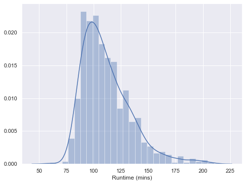
Film durations
sns.distplot(movies['Runtime (mins)'])
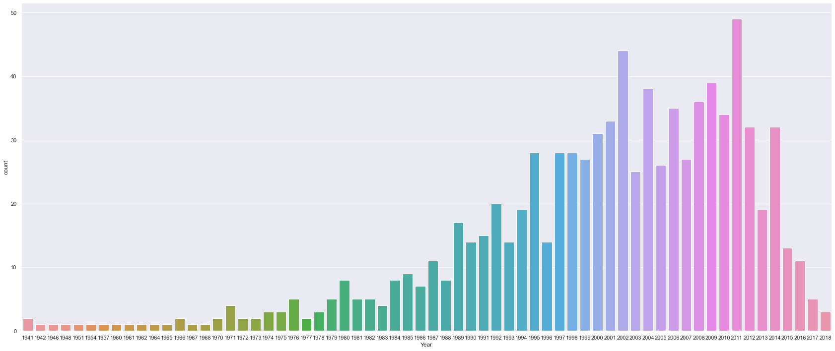
Film Release Years
sns.catplot(x="Year", kind="count", data=movies, height=10, aspect=21/9)
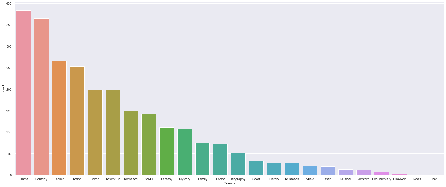
Film genres
genres = movies['Genres'].astype('str').tolist()
genres = list(map(lambda x: x.split(','), genres))
genres = sum(list(genres), [])
genres = list(map(lambda x: x.strip(), genres))
genres = list(map(lambda x: [x], genres))
genres = pd.DataFrame(genres, columns=['Genres'])
sns.catplot(x="Genres", kind="count", data=genres, height=9, aspect=21/9, order = genres['Genres'].value_counts().index)
Directors
directors = movies['Directors'].astype('str').tolist()
directors = list(map(lambda x: x.split(','), directors))
directors = sum(list(directors), [])
directors = list(map(lambda x: x.strip(), directors))
directors = list(map(lambda x: [x], directors))
directors = pd.DataFrame(directors, columns=['Directors'])
directors = directors.groupby(['Directors']).size()
directors = directors.reset_index(name='size')
directors = directors.sort_values(['size'], ascending=False)
directors.head(10)
| Directors | size | |
|---|---|---|
| 514 | Steven Spielberg | 15 |
| 453 | Robert Zemeckis | 10 |
| 111 | David Fincher | 8 |
| 345 | Martin Scorsese | 8 |
| 415 | Peter Jackson | 7 |
| 423 | Quentin Tarantino | 7 |
| 256 | John Hughes | 7 |
| 85 | Christopher Nolan | 6 |
| 464 | Ron Howard | 6 |
| 155 | Ethan Coen | 6 |
What’s the perfect film for me?
Based on frequent attributes: It looks like that would be a Drama or Comedy, directed by Spielberg, made in 2011, that is about 100 minutes long! ‘War Horse’, anybody?
If we base it on rating, by restricting this to just films I rated >= 8: A Drama, directed by Spielberg, made in 1999, that’s 120 minutes long. Perhaps, ‘Saving Private Ryan’?
This however would be an interesting small ML project: to create a model to predict a numeric rating for a given film, based on my previous ratings.