Multiclass Image Classification with CNNs

Introduction

In this post, I’ll present the analysis and processing of an images dataset, and the training and application of Convolutional Neural Network (CNN) models (using PyTorch) for the purpose of multiclass classification of the dataset. The dataset is the ‘The Simpsons Characters Dataset’ [1] (obtained from Kaggle [1]), and contains still images of different characters taken from the television show The Simpsons [2].

The goal of the analysis and modelling, and hence the problem statement, is: Given the Simpsons Characters image dataset, how accurately can the characters in the images be correctly identified?

The accompanying code and data repository can be found here.

The Data

Background & Overview

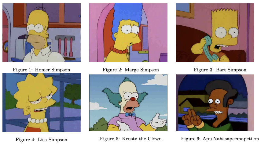
The full image dataset contains ~22,000 still images of 42 different cartoon characters. The images are taken from the popular, animated, American television show The Simpsons [2]. As of 2023, the show has broadcast 760 episodes across 35 ‘seasons’ since 1989 [3]. Over this time, (human) fans of the television show have become familiar with the characters and can easily identify them. Figures 1-6 below show example images from the dataset, with the captions indicating the respective character’s name. Each image in the dataset contains only one character.

For the purposes of this analysis, a sub-sample of the data was selected. This is because, given its size, using the full dataset presents a computational challenge: training a model on it would take impractically long. Instead a sub-sample of ~⅓ of the size of the full sample was taken. This subsample contains 8,363 images of 6 characters.

These characters are (short names in brackets): Homer Simpson (Homer), Marge Simpson (Marge), Bart Simpson (Bart), Lisa Simpson (Lisa), Krusty the Clown (Krusty) and Apu Nahasapeemapetilon (Apu). These 6 characters are the same ones shown in Figures 1-6. Further detail on this sub-sampling is described in the Pre-Processing section. Note: in the Github repo, the dataset was further sub-sampled to reduce the size to under 100mb; again, this is described in the Pre-Processing section.

Dataset Challenges

There are a number of challenges to working with this dataset, which fall into two categories: (1) complexity due to the quality of the images, and (2) intrinsic complexity of the content of the images.

(1) The quality of the images introduces complexity:

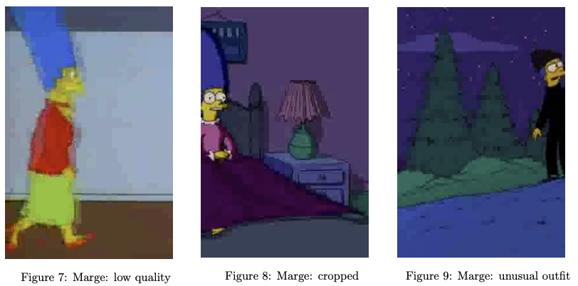
• Firstly, the images vary in both size and resolution. For example, Figure 7 shows a low resolution noisy image (288 × 432 pixels, 72 pixels/inch).
• Secondly, there is varying character cropping and centering. For example, Figure 8 shows the character is partially cropped, possibly losing useful information. In Figure 9 the character is not centred, and so there is possibly a lot of irrelevant information included in the image.

(2) There is intrinsic complexity to the content of the images:

• For example, there is significant variation between images: the characters change outfits, or the characters appear against varying backgrounds (compare Figure 7 with Figure 9).
• There are also similarities that may make it difficult to discern between characters: the most obvious of which is the show’s hallmark animation style wherein most characters are yellow skin tone and circular eyes [3] (consider Figures 1, 2, 3 and 4).

Pre-Processing

The full dataset comprises two sets of images:

• Training set: ~21,000 images of 42 characters
• Test set: ~1,000 images of 20 characters (a subset of the characters in the training set)

The data was already mostly organised into a training and test set, however some movement and manipulation of the filenames and directories was required in order to facilitate loading and processing by the Pytorch library [6]. One such shell script for performing these file operations is included in the Github submission for completeness (script_to_move_and_rename_test_data_files.sh) .

As mentioned in the Data Background & Overview section, a subsample of this dataset was used for this analysis. The sub-sample was taken by selecting 6 characters, and using all of their training and test images. The analysis sub-sample thus comprises:

• Training Set: 8,063 images of 6 characters
• Test Set: 300 images of 6 characters

The 6 characters in the sub-sample were selected in following way, and represent an interesting subset of characters:

• Homer, Marge, Bart, and Lisa were selected as they are all important characters from the show’s eponymous, central family The Simpsons. Additionally, analysis by Schneider (2016) [4] (see Figure 10) shows that they are also the 4 top characters in the show based on number of words spoken.

• Krusty was selected as he is also a top-10 character [4] and, more interestingly, this character’s appearance strongly resembles that of Homer. This was a deliberate design decision by the show’s creators [7]. Classifying two characters that resemble each other might provide an interesting challenge to the model.
• Apu was selected as he is one of the show’s few characters who does not have ‘yellow’ skin tone (a hallmark of the the show’s animation style). Again, this character’s unique skin tone might provide an interesting challenge to model, and give some insight into which image features the model learns from.

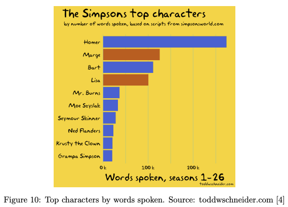
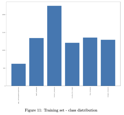
Figure 11 shows the distribution of character images in the training set. The Training set exhibits some class imbalance (e.g. Homer has ~4x as many images as Apu). In contrast, the Test set is balanced: 50 images each for the 6 characters.

Note that in the final accompany Github repo, further subsampling was performed to bring the submitted dataset to under 100mb in size (image_data_subsample_subset.zip) (Training Set: 2,980 images, Test Set: 300 images). This ‘sub-sub-sample‘ contains images of the same 6 characters.

Note however that the analysis in this post uses the analysis subset of 8363 images, and not the Github repo sub-sub-sample.

The images in the dataset were pre-processed in 4 different ways; those 4 approaches are described below:

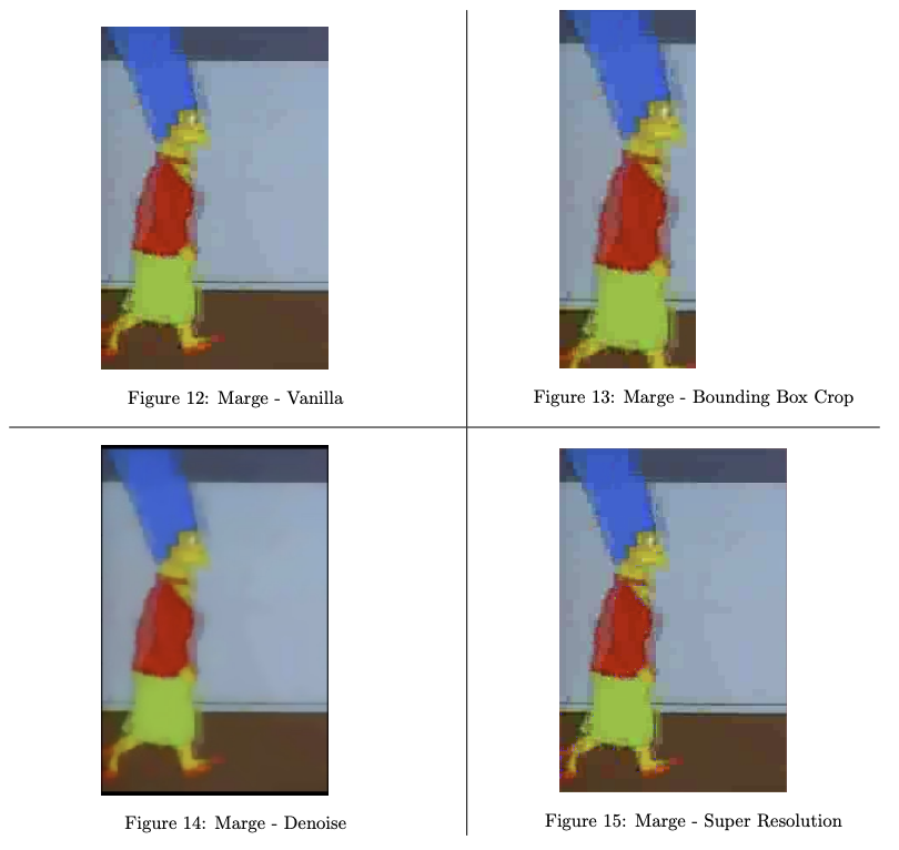
1. Pre-processing approach 1 ‘Vanilla’: Resize all the images to 255x342 pixels, keeping the 4x3 (television broadcast) aspect ratio.
2. Pre-processing approach 2 ‘Bounding Box Crop’: Apply pre-processing approach 1, plus: Crop the images using the bounding box coordinates in the ’annotations’ file supplied in the dataset. One of the bounding box coordinates was found to be erroneous and was removed.
3. Pre-processing approach 3 ‘Denoise’: Apply pre-processing approach 1, plus: Denoise the image using the denoise tv chambolle function from skimage [8].
4. Pre-processing approach 4 ‘Super Resolution’: Apply pre-processing approach 1, plus: Improve the image resolution by using the ninasr b0 ‘super-resolution’ neural network model from the torchSR package [9].

As a final step in all the pre-processing approaches, all of the images are converted to Pytorch tensors, for inputting to the model.

To implement the pre-processing steps described above, a custom Pytorch ImageFolder class was defined ImageFolderWithPath, which not only loads the image but also captures the path name (the paths include the character names which are used as the class names in the classification model), and applies the pre-processing transformations.

Figures 12-15 below show the results of the different processing approach on the same image.

Modelling

Restating the problem statement: Given the Simpsons Characters image dataset, how accurately can the characters in the images be correctly identified?. This is formulated here as a multi-class classification problem, where the character names are the classes, and the images are to be classified as belonging to a particular class if the image depicts that particular character. Each image contains only one character.

To perform the classification task, a Convolutional Neural Network (CNN) was constructed, using pytorch. CNNs are a popular deep learning technique with many applications but are particularly useful in image classification tasks. A CNN was developed with the following layers:

• Input layer: Images are inputted as tensors (following pre-processing)
• Layer 1 (hidden layer): Applies: a 2D convolution over the image, followed by Batch Normalization, followed by a ReLU (rectified linear unit) function, and finally 2D max pooling.
• Layer 2 (hidden layer): The same as layer 1, but on the output from layer 1
• Fully connected layer: Applies a linear transformation.
• Dropout: Applies the dropout regularisation technique, with probability 0.5.

As an illustration, Figures 16-18 below show an example original input image, and the intermediate outputs of the network’s hidden layers. (This was taken from ‘Vanilla’ model described below).

The image dataset was processed separately in each the 4 ways described in the Pre-Processing section, and then inputted into 4 separate CNNs. Thus, there are 4 models that all have the same model architecture but were trained on input data pre-processed in 4 different ways:

1. Model 1: Referred to as ‘Vanilla’. This model was inputted with the image dataset where only basic pre-processing applied, e.g. resize but keep 4x3 ratio, converting the images to a tensors (‘Pre-processing Approach 1’).
2. Model 2: Referred to as ‘Bounding Box Crop’. This model was inputted with the image dataset with all of the same basic pre-processing steps as Model 1, plus the images were cropped using the bounding box annotations supplied with the dataset (‘Pre-processing Approach 2’).
3. Model 3: Referred to as ‘Denoise’. This model was inputted with the image dataset with all of the same basic pre-processing steps as Model 1, plus the images were denoised (‘Pre-processing Approach 3’).
4. Model 4: Referred to as ‘Super Resolution’. This model was inputted with the image dataset with all of the same basic pre-processing steps as Model 1, plus the resolution of the images was enhanced using a super resolution model (‘Pre-processing Approach 4’).

For each of the models: The training data was loaded in batches of 100, and training was performed for 5 epochs over the training data. The number of epochs was chosen to be 5 as to provide a balance between model performance (with respect to test accuracy) and to complete training within a practical length of time.

Training took approximately 2 hours on a Macbook Pro (2020) laptop with the following specs:

• Processor: 2 GHz Quad-Core Intel Core i5
• Graphics: Intel Iris Plus Graphics 1536 MB
• Memory: 16 GB 3733 MHz LPDDR4X
• Operating System: macOS 14.2.1

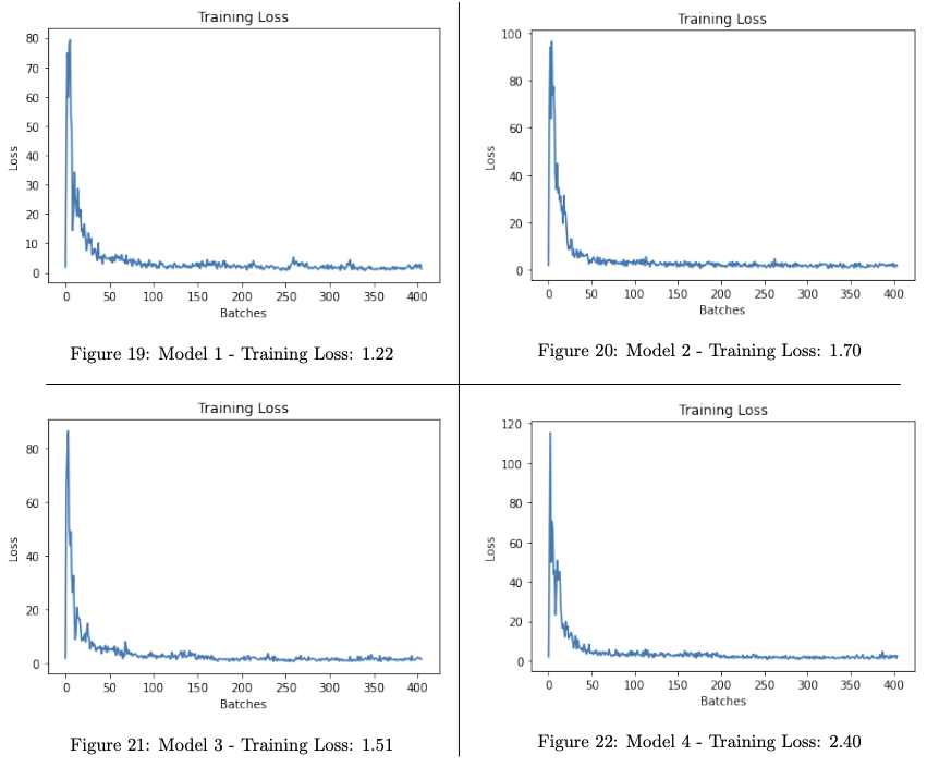
Figures 19-22 show, for each of the models, the training loss over the course of the batches. We can see that they all converged fairly quickly, within ~50 batches. The captions give the training loss for the final batch. Model 4 had the highest Training loss but, as explained in the later Results & Interpretation section, generalised well to the Test set and demonstrated a high accuracy and f1-score.

Results & Interpretation

The 4 models were evaluated against a Test set of 300 unseen images: 50 images for each of the 6 characters.
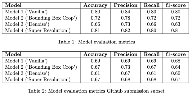
        Table 1 compares the models based on a number classification evaluation metrics: Accuracy, Precision, Recall, and f1-score. Micro averages are provided for those latter 3 metrics - since there is no class imbalance in the test data and all classes are of equal importance. The numbers are given to 2 d.p. We can see that Models 1 and 4 performed the best across the metrics: Model 4 had the highest Accuracy and f1-score (both 0.81), Model 1 had the highest Precision (0.84), and both models had equal Recall (0.8). In contrast, Models 2 and 3 performed less well, and specifically Model 2 performed the worst across all metrics.
        The relative poor performance of Models 2 and 3 suggests that removing perceived (but not actually) irrelevant information from an image (Model 2 - bounding box cropping), or removing noise (Model 3 - denoising) may in fact harm the quality of the image and information therein, and thus affect model performance.
        The slightly improved Accuracy and f1-score of Model 4 suggests that improving the resolution of the images can improve model performance, however the improvement is small and so may not justify the increased model training time.
        Table 2 shows the metrics for the Github subset (included here for completeness). We can see that the models’ performance is worst on this subset than for the larger sub-sample - which may be explained by having less data to train on and learn from. However the relative performances of the models remains similar: Model 3 is the worst, and Model 1 and Model 4 perform similarly well.

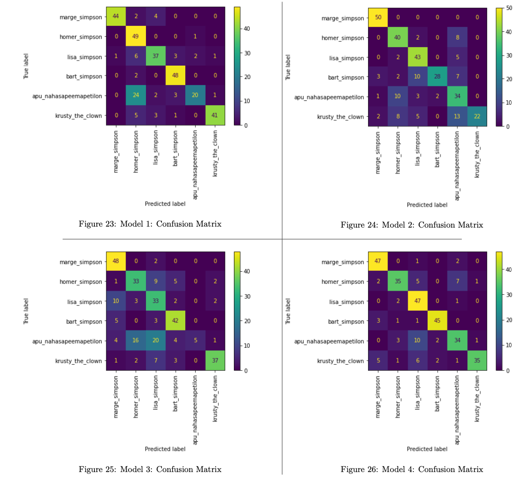
Figures 23-26 show the confusion matrices for the each of the models.
        Across all 4 models, it appears that the character Apu is the most misclassified. This is interesting: Apu is unique among the characters in the dataset in that he is the only one without (mostly) yellow skin tone, which intuitively might suggest that correctly classifying an image of him would be easier. However, this colour information may have been missed/lost by the model (e.g. see Figures 17 and 18 for intermediate model outputs), thus reducing the ability to discern his appearance without that information.
        In contrast, Marge was the least misclassified character across all models - perhaps the unique shape of the character’s head/hair facilitates classification.
        We can also see that Krusty was (as expected) occasionally misclassified as Homer by all of the models, however this was not the most common misclassification: e.g. Model 2 misclassified Krusty as Apu more times than it did Krusty as Homer (13 vs 8 times). This suggests that the animator’s intended similarity between Homer and Krusty did not dominate the features that the models learned.

The results of this analysis can be compared to the results from another project by the dataset’s curator (Attia 2017) [5]. In that project, the f1-score, precision and recall were all 0.9. That was achieved through:

1. Using the full dataset of 22k images
2. Implementing a more sophisticated and complex deep learning neural network architecture with more layers
3. Training for more epochs (200 epochs).

Conclusion

In conclusion, this analysis and report has shown that, through careful pre-processing of image data and appropriate model selection and training, it is possible to achieve reasonably good performance in the multi-class classification problem of identifying characters in still images taken from the television show The Simpsons.

An accuracy and f1-score of 0.81 were achieved through a combination of applying super-resolution to the images in the pre-processing stage, and training a convolutional neural network with 2 hidden layers for 5 epochs over the data. It was shown that applying image cropping and denoising could have a negative impact on classification performance.

Further analysis could explore how to improve classification performance further, for example by combining these pre-processing techniques, or training the model for more epochs, or adding more layers to the network.

---

References

1. Attia, A. (2017). The Simpsons Characters Dataset
2. Groening, M., et al. (1989) The Simpsons. Fox Broadcasting Company.
3. Wikipedia. (2023) The Simpsons.
4. Schneider, T. (2016). The Simpsons by the Data
5. Attia, A. (2017). The Simpsons characters recognition and detection using Keras (Part 1).
6. Paszke, A., et al. (2019) Pytorch: An imperative style, high-performance deep learning library. Advances in neural information processing systems 32.
7. Caroll, L. (2007). ‘Simpsons’ Trivia (MTV website archived).
8. Van der Walt, S. et al. (2014) scikit-image: image processing in Python. PeerJ, 2, p.e453.
9. Gouvine, G. (2021). torchSR.