Generating Audio of Spoken Digits, with VQ-VAE and LSTM models

5 minute read

Introduction

This post presents an analysis of the Free Spoken Digit Dataset (FSDD) (an “audio/speech dataset consisting of recordings of spoken digits” [1]) and the use of this dataset in the development of two machine learning models (a VQ-VAE model and an LSTM model) which are combined for the purpose of generating new samples of audio of spoken digits.

Exploratory Data Analysis

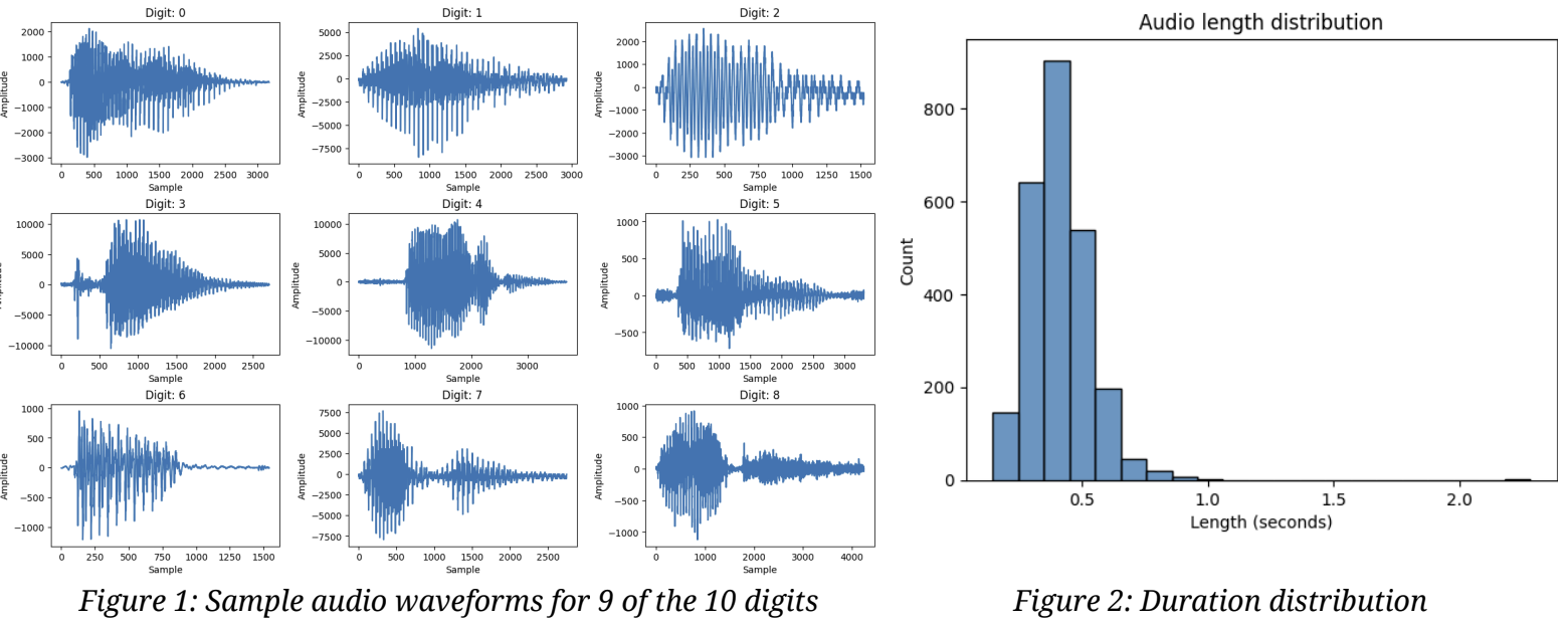
The FSDD dataset consists of 2500 audio recordings, by 5 speakers, of 10 different digits (where there is 50 recordings per digit per speaker). These recordings are in wav files with a 8kHz sample rate, and are of variable duration.

Figure 1 below shows the audio waveforms of a sample recording for 9 of the 10 digits; we can see that recordings of different digits by different speakers have different shaped waveforms. Figure 2 shows the distribution of durations of the recordings; we can see that most recordings are quite short - indeed 99% are shorter than 0.78 seconds.

Fig1-2

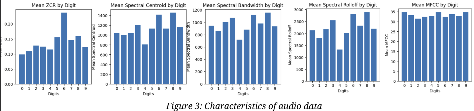
Audio characteristics of the samples were computed using librosa: Zero-Crossing Rate (ZCR), Spectral Centroid, Spectral Bandwidth, Spectral Rolloff, and Mel-frequency cepstral coefficients (MFCC). Figure 3 below summarises the means of these values for each digit. We can see for example that the digit ‘6’ has a distinctive mean ZCR value that is much higher than for other digits. Similarly, we see that the digit ‘5’ has a mean Spectral Rolloff value that is much lower than the other digits.

Fig3

Modelling & Results

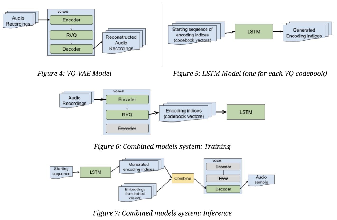
The goal was to develop models for the purpose of generating new samples of audio of spoken digits. To achieve this, two models were developed and their functionality combined into one system for generating new audio samples. These two models are referred to as model A and model B, respectively, and are described in detail below.

At a high-level: model A (Figure 4) is a Vector-Quantized Variational Autoencoder (VQ-VAE), similar to that introduced in [2], and is used to learn efficient encodings of the audio data. Model B (Figure 5) is an LSTM model that is trained on model A’s output (indeed, one LSTM per VQ codebook), and is used to generate new encoding sequences; these sequences are in turn reconstructed into listenable audio clips using model A’s decoder. Figures 6 and 7 below show the training and inference processes of the combined model system.

Fig4-7

Model A: VQ-VAE

The FSDD data was processed by first extracting the audio component (for each clip, this is a 1-D array representing amplitude over time), then filtering out very long and short clips, then zero-padding the remaining clips to 1 second duration (uniform size to simplify code). The data was then split into training and test sets, and finally shuffled and batched.

The training data was used to train the ‘VQ-VAE’ model. The model has 3 components:

An encoder comprising three 1-D convolutional layers
An RVQ-VAE layer comprising Nq VQ-VAE layers
A decoder comprising three 1-D convolutional transpose layers

The model was trained using customised training logic that optimised for loss defined as loss = reconstruction loss + RVQVAE loss.

Various settings for the hyperparameters were explored as part of experimentation, specifically:

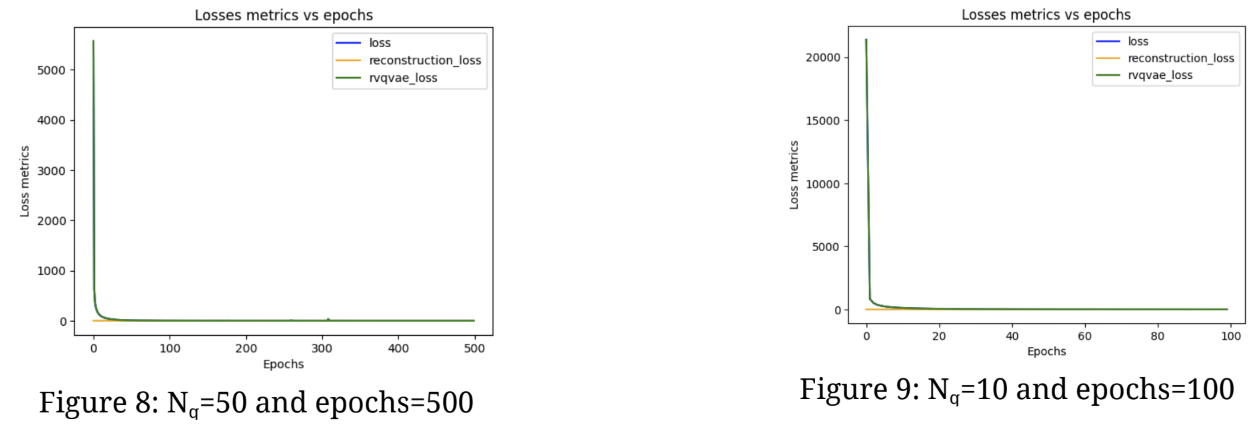
The hyperameter Nq that controls the number of codebooks in the RVQ-VAE layer (values: 5, 10, 50).
The number of epochs that training is conducted for (values: 30, 100, 500).

Higher Nq values and extended training epochs resulted in improved outcomes; however, this led to longer training times. To assess the results, a combination of training loss comparisons and subjective manual auditory evaluations was used (audio samples can be found in the notebook). The optimal combination achieved an overall loss of 0.0761 (reconstruction loss of 0.0349 and an RVQVAE loss of 0.0412). With a Nvidia T4 GPU on Google Colab, this setup took approximately 1.5 hours to train. Figures 8 and 9 compare the loss curves for two sets of hyperparameter settings, showing that higher Nq values result in lower loss in fewer epochs.

Fig8-9

Model B: LSTM model

The audio training data was once again processed by (forward) passing it through the trained VQ-VAE model’s encoder and RVQ-VAE layers (notably, not the decoder) to generate the corresponding Nq encodings (one for each codebook in the RVQ-VAE). These encodings were then used to train Nq LSTM models.

Each LSTM model comprises:

An embedding layer with an input dimension of 64 (same as the codebook vectors), and an output dimension of 64
Two LSTM layers with 256 units
A Dense output layer with softmax activation that outputs probabilities over the possible tokens (additional logic later chooses the token with the highest probability)

The model was trained using the standard Tensorflow fit method and training logic, with 10% of the training data used as a validation set. Various settings for the hyperparameters were explored as part of experimentation, including a different number of LSTM layers and different dropout rates (ultimately 2 and 0.2 was chosen, respectively), while trading off against training duration.

Performance was measured using training and validation loss and accuracy. While performance against training/validation was good (~70% accuracy across the LSTM models), the performance against the unseen test set was not good: it was found that the model outputted constant vectors of the same code. This unfortunately leads to poor quality reconstructed audio. With more time, this poor performance could be investigated.

Future Work

With more time, future work in this direction could involve:

Explore the use of representing audio as an image instead of a series of amplitude values over time, possibly by combining graphical representations of audio characteristics (i.e. spectrograms and MFCCs) into an image. Modify the encoder and decoder of the VQ-VAE to use 2-D convolutional layers accordingly. This was partially attempted in the notebook, but futher implementation is needed to convert the reconstructed image representation back to audio (this may be challenging).
Train both models for more epochs to achieve better performance (lower loss and higher accuracy). Due to time limitations and available resources, training was conducted for fewer epochs than desired.
Investigate and optimise the hyperparameters of both models, especially the LSTM. Conduct more experimentation to find the optimal settings for improved performance.

Conclusion

In conclusion, this report demonstrates the feasibility of generating new samples of audio data by first training a VQ-VAE model to learn efficient codings of the audio data, and then using those encodings to train an LSTM model to generate new encodings, which can in turn be decoded into listenable audio. While the final audio clips generated are not of the highest quality, the report details possible directions for future work to pursue better performance.

References

Zohar J., et al. (2018). Jakobovski/free-spoken-digit-dataset: v1.0.8 (v1.0.8). Zenodo.
van den Oord, A., Vinyals, O. & Kavukcuoglu, K. (2017). Neural discrete representation learning. Proceedings of the 31st International Conference on Neural Information Processing Systems, 6309-6318.

Note: This post is based on a report written for an assignment as part of my degree in Machine Learning & Data Science at Imperial College London. The assignment was part of Deep Learning module taught by the highly knowledgable and supportive Dr. K Webster (all credit due for the assignment setting, the goals and objectives of the modelling, and the selection and provision of the dataset).

Mansour Ahmed